Scrape typhoon data and visualize on an interactive geographic map
Using R to scrape data and plotly to visualize typhoon Kompasu
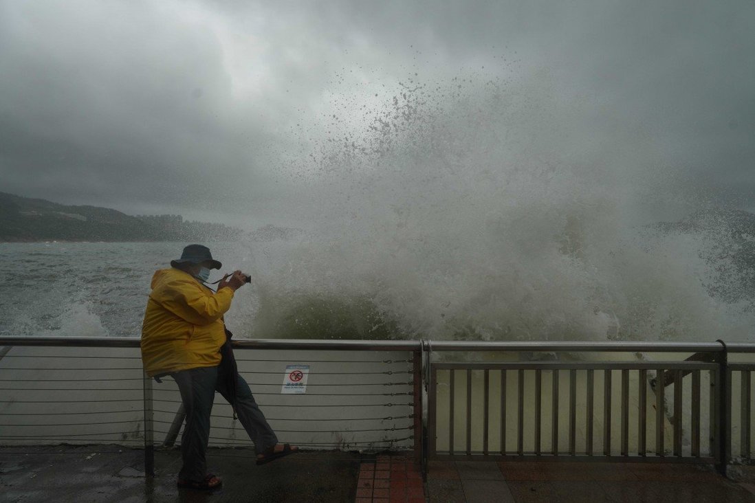 Image credit: SCMP
Welcome
In the SMU Master of Professional Accounting elective course Programming with Data, we use some typhoon data to predict shipping delays. Although we don’t cover in class how we scrape data from websites, I strongly encourage you to spare some time to read this post on web scraping using R. You may have already read my other post on scraping tables. I am mainly using package:rvest and you must read the Web scraping 101.
Scrape typhoon data
Before we start, I assume you have some basic understanding of HTML element as shown in the following image.
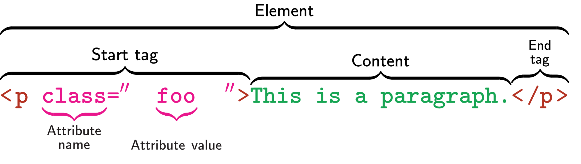
The basic idea of web scraping is to find the content you want to get. For example, in the above image, if you want to get the content This is a paragraph, you can find the HTML element by searching the tag name p. It is possible that there are some other elements which also use p tag and do not contain the contents you want. So you may use the class value foo to locate the elements which contains the data you want.
In short, you should try to inspect the HTML codes and try to identify the HTML elements you want using the tag names and attribute names. Of course you may also want to get the value of attribute and you should do the same.
Typhoon Kompasu
There is an active tropical cyclone that is affecting the Philippines, Taiwan, and Southeast China. The typhoon is named as 24W in the U.S., Kompasu in Japanese, 圆规 in Chinese and Maring in Philippines. It was originated from an area of low pressure east of the Philippines on October 7, 2021. We will try to get its location data and plot it on a geographic map.
so, how do typhoon get their names? Read here
Kompasu has already killed dozens in Philippines and Hong Kong. Let’s pray that there will be no more casualties.
The Satellite Products and Services Division of the National Environmental Satellite, Data, and Information Service (NESDIS) of the U.S. provides all typhoon archival data. Our task now is to scrape the 2021 typhoon data.
Get Typhoon data address
From the website, you may notice that each typhoon data is stored in a separate text file (.txt). You may use some mass downloading software to download all the files directly. Here I am trying to use R package:rvest to scrape all the files automatically.
My steps are as follows:
- find the address for all text files
- download the files and merge them into a data frame
Let’s start!
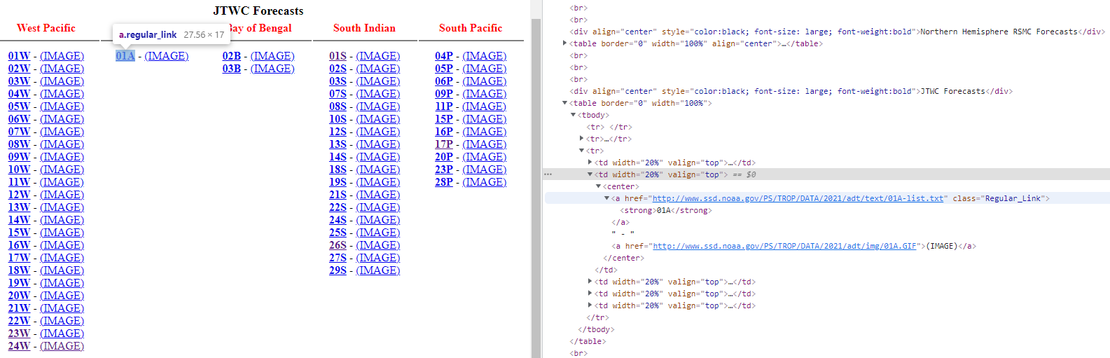
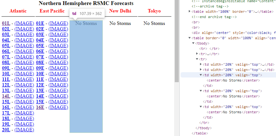
You need to first Inspect the page by right click on any of the typhoon name such as 24W. You will then see the HTML source code. Look around and try to identify the HTML elements which contain the file address.
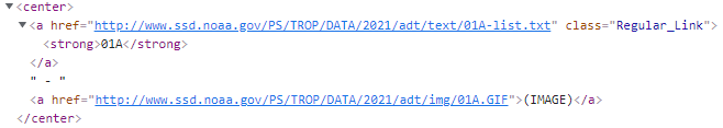
From the Inspect image above, it seems all the file addresses and also typhoon names are within the center tag, as shown below. The element contains the following three things:
- attribute
hrefand its value which is the file address we are looking for - attribute
classwith its valueRegular_Linkwhich can be used to identify this particular element as there are some other elements which also havecentertag. - tag
strongand its content01Awhich is the name of the typhoon. - there is another attribute
hreffor image but we are not interested in it
 Now let’s begin our code to scrape the data. We will use the popular
 package:tidyverse for data manipulation and the package:rvest for web scraping. The very first step is to read the HTML page using read_html() and then look for the elements which is identified by tag center. The html_elements() function will search for all the HTML elements which contain the center tag, ie, anything between the start tag <center> and end tag </center>.
library(tidyverse)
library(rvest)

# read a html file into xml object to be handled by rvest
content <- read_html("https://www.ssd.noaa.gov/PS/TROP/2021/adt/archive.html")

# figure out which part of the data you need by Inspect the website
content_center <- content %>%  html_elements("center")
Under each element, we need to collect two data: the file address which is the value of attribute href and typhoon name which is the content of tag strong. We can read each of them and then build a data frame using the data.frame() function. Note the difference between html_elements() and html_element(). The formal is to search for all the elements and the latter is to search one element one by one.
html_attr(): get the value of the given attribute namehtml_text2(): get the content of a given taghtml_text()can also be used but it is better to usehtml_text2()as shown here
table <- data.frame(
  urls = content_center %>% html_element(".Regular_Link") %>% html_attr("href"),
  typhoon_name = content_center %>% html_element("strong") %>% html_text2()
) %>% filter(!is.na(urls))
Also note that there are some missing values (three records) as there are no typhoon under three regions: Central Pacific, New Delhi and Tokyo. It will be recorded as NA automatically.
Let’s see what data we got.
head(table)
##                                                              urls typhoon_name
## 1 http://www.ssd.noaa.gov/PS/TROP/DATA/2021/adt/text/01L-list.txt          01L
## 2 http://www.ssd.noaa.gov/PS/TROP/DATA/2021/adt/text/02L-list.txt          02L
## 3 http://www.ssd.noaa.gov/PS/TROP/DATA/2021/adt/text/03L-list.txt          03L
## 4 http://www.ssd.noaa.gov/PS/TROP/DATA/2021/adt/text/04L-list.txt          04L
## 5 http://www.ssd.noaa.gov/PS/TROP/DATA/2021/adt/text/05L-list.txt          05L
## 6 http://www.ssd.noaa.gov/PS/TROP/DATA/2021/adt/text/06L-list.txt          06L
Great! We now have all the files’ address and the names of all typhoon. We can now start to read each text file and merge them into one data frame.
Examine data file format
I am going to use two functions to read text files.
readLines(): read each line of text as a character and return a vector of all lines of characters. Check the following example. It reads the text file into a vector of character which contains all the 183 lines of text. Each element of the vector represents one line of text. As you can see, the first four lines are header information; the last three lines are footer information, including one blank line. Lines between are the typhoon data.
lines <- readLines("http://www.ssd.noaa.gov/PS/TROP/DATA/2021/adt/text/24W-list.txt")
str(lines)
## chr [1:186] "===== ADT-Version 8.2.1 =====" ...
head(lines)
## [1] "=====  ADT-Version 8.2.1 ====="
## [2] "                  ----Intensity--- -Tno Values-- ---Tno/CI Rules---  -Temperature-                    "
## [3] "           Time         MSLP/Vmax   Fnl Adj Ini   Cnstrnt Wkng Rpd    Cntr   Mean   Scene  EstRMW   MW   Storm Location  Fix"
## [4] "   Date    (UTC)   CI  (CKZ)/(kts)  Tno Raw Raw    Limit  Flag Wkng  Region  Cloud  Type    (km)  Score   Lat     Lon    Mthd    Sat   VZA  Comments"
## [5] "2021OCT10 130000  2.5  990.7  35.0  2.5 2.5 2.5  NO LIMIT  OFF  OFF   13.31 -33.24  CRVBND   N/A    N/A   18.44 -126.51  FCST    HIM-8 27.0 "
## [6] "2021OCT10 133000  2.5  990.7  35.0  2.4 2.3 2.0  0.2T/hour  ON  OFF   15.55 -36.89  CRVBND   N/A    N/A   18.51 -126.41  FCST    HIM-8 27.1 "
tail(lines)
## [1] "2021OCT14 080000  1.5 1003.0  25.0  1.5 1.5 1.5  NO LIMIT   ON  OFF   10.90   6.24  SHEAR    N/A   -2.0   19.24 -106.15  FCST    HIM-8 45.0 "
## [2] "2021OCT14 083000  1.5 1003.0  25.0  1.5 1.5 1.5  NO LIMIT  OFF  OFF    8.42   5.46  SHEAR    N/A   -2.0   19.25 -106.07  FCST    HIM-8 45.1 "
## [3] "2021OCT14 090000  1.5 1003.0  25.0  1.5 1.5 1.5  NO LIMIT  OFF  OFF   11.16   4.57  SHEAR    N/A   -2.0   19.26 -105.99  FCST    HIM-8 45.2 "
## [4] "Utilizing history file /home/Padt/ADTV8.2.1/history/24W.ODT"
## [5] "Successfully completed listing"
## [6] ""
read_fwf(): read a fixed width file. If you check some text files on the website, you may notice that they are in the same format with the same width. This make file parsing very efficient because every field is in the same place in every line. This type of file is different from.csvfile as it does not have a common delimiter such as,and;to separate columns. The downside is that you have to specify the width for each column.
There is one more thing to handle before we read all the text files. The width of files in the Southern Hemisphere is different from the rest, including one more column of BiasAdj under the header Intensity.
lines <- readLines("https://www.ssd.noaa.gov/PS/TROP/DATA/2021/adt/text/23U-list.txt")
head(lines)
## [1] "=====  ADT-Version 8.2.1 ====="
## [2] "                  --------Intensity------- -Tno Values-- ---Tno/CI Rules---  -Temperature-                    "
## [3] "           Time         MSLP/MSLPLat/Vmax   Fnl Adj Ini   Cnstrnt Wkng Rpd    Cntr   Mean   Scene  EstRMW   MW   Storm Location  Fix"
## [4] "   Date    (UTC)   CI  (DvT)/BiasAdj/(kts)  Tno Raw Raw    Limit  Flag Wkng  Region  Cloud  Type    (km)  Score   Lat     Lon    Mthd     Sat   VZA  Comments"
## [5] "2021APR06 013000  2.5 1005.0   +0.0   35.0  2.5 2.5 2.5  NO LIMIT  OFF  OFF  -11.33 -31.67  CRVBND   N/A    N/A  -16.48 -105.33  FCST    HIM-8 44.6 "
## [6] "2021APR06 020000  2.5 1005.0   +0.0   35.0  2.4 2.3 2.1  0.2T/hour  ON  OFF   14.65 -38.55  CRVBND   N/A    N/A  -16.49 -105.35  FCST    HIM-8 44.6 "
Luckily this is the only difference of all the files. Otherwise we have to do more manual work. In the age of machines, data format (which is part of data governance & quality) is vital for efficient usage of data.
After careful examinations of all file headers, we define two headers and column width as follows. We will use different header/width for different files later.
header1 <- c("date", "time", "intensity_ci", "intensity_mslp",
             "intensity_vmax", "tno_fnl", "tno_adj", "tno_ini", "constrnt",
             "wkng", "rpd", "temp_ctr", "temp_mean", "scene","est_rmw",
             "mw","lat","lon","mthd","sat","vza","comments")
widths1 <- c(9, 7, 5, 7, 6, 5, 4, 4, 10, 5, 5, 8, 7, 8, 7, 6, 8, 8, 6, 9, 5, NA)
header2 = header <- c("date", "time", "intensity_ci", "intensity_mslp",
                      "intensity_mslpplat", "intensity_vmax", "tno_fnl",
                      "tno_adj", "tno_ini", "constrnt", "wkng", "rpd",
                      "temp_ctr", "temp_mean", "scene", "est_rmw", "mw",
                      "lat", "lon", "mthd", "sat", "vza", "comments")
widths2 <- c(9, 7, 5, 7, 8, 6, 5, 4, 4, 10, 5, 5, 8, 7, 8, 7, 6, 8, 8, 6, 9, 5, NA)
Read all data files
We will use the for loop to read all the files. The algo for reading one file is as follows:
- read the file into a vector using the
readLines()function - check if
BiasAdjis in line 4, assign a different header and width - read the data from line 5 to the end except for the last 3 lines
- bind the rows to the previous file
The for loop code is as follows. Note that I created an index q which will be printed out for every loop. The number of loop should be the total number of files it reads, which is 107. For the interest of space, I did not show the code printing output.
The first is an indicator of first loop, which will be used to determine when to bind the rows with previous files (ie, first file no need to bind). You may also use the other technique for reading and binding multiple files.
first <- TRUE
q <- 1

for(url in table$urls) {
  print(paste("reading typhoon data:", q))
  lines <- readLines(url)
  name <- table$typhoon_name[q]
  # check if "BiasAdj" in line 4 -- if so, need an extra column!
  if(length(grep("BiasAdj", lines))) {
    widths <- widths2
    h <- header2
  } else {
    widths <- widths1
    h <- header1
  }

  lines <- lines[5:(length(lines)-3)]

  data <- read_fwf(paste0(lines, collapse="\n"),
                   fwf_widths(widths, col_names = h),
                   na = "N/A")
  data$est_rmw <- as.character(data$est_rmw)
  data$typhoon_name <- name
  if(first) {
    first = F
    typhoon <- data
  } else {
    typhoon <- bind_rows(typhoon, data)
  }
  q <- q + 1
}

# write.csv(typhoon, "typhoon.csv", row.names = F)
Plot the geographic map

Let’s try to plot the typhoon data on a simple geogrpahic map using the package:plotly.
The first step is to extract the Kompasu typhoon data. As we shared at the beginning, the name for Kompasu in the data is 24W. Somehow I found the longitude data is negative and I changed it to positive which will show the correct location of the typhoon on the map. Let me know if my understanding is wrong here. Apparently I need to learn more knowledge in geography.
typhoon_Kompasu <- typhoon %>%
  filter(typhoon_name == "24W") %>%
  mutate(lon = -1 * lon,
         typhoon_name = "24W: Kompasu")
Now we will use the package:plotly for plotting. I also introduce you the package:RcolorBrewer for color palettes. I don’t have to use the color palettes here as I have plotted one typhoon only. But it is good to know that we can use the package for color management in R. I will make a simple plot what we do in class.
In the following code, we define a color palette using the brewer.pal(). We also define a geographic map object geo. You have to refer to the geo projection manual for more details.
library(plotly)
library(RColorBrewer)

palette = brewer.pal(8, "Dark2")[c(1, 3, 2)]

geo <- list(
  showland = TRUE,
  showlakes = TRUE,
  showcountries = TRUE,
  showocean = TRUE,
  countrywidth = 0.5,
  landcolor = toRGB("grey90"),
  lakecolor = toRGB("aliceblue"),
  oceancolor = toRGB("aliceblue"),
  projection = list(
    type = 'orthographic', #check https://plot.ly/r/reference/#layout-geo-projection
    rotation = list(
      lon = 100,
      lat = 1,
      roll = 0
    )
  ),
  lonaxis = list(
    showgrid = TRUE,
    gridcolor = toRGB("gray40"),
    gridwidth = 0.5
  ),
  lataxis = list(
    showgrid = TRUE,
    gridcolor = toRGB("gray40"),
    gridwidth = 0.5
  )
)
Finally, we are here to plot the typhoon on the map using the plot_geo() function. This is a bit simple and ugly and I trust you have much better design taste than me. Share with me your code in the below comment box if you can plot a better one.
p <- plot_geo(colors = palette) %>%
  add_markers(data = typhoon_Kompasu,
              x = ~lon,
              y = ~lat,
              color = ~typhoon_name,
              text = ~paste("Name", typhoon_name, "</br>Time: ", date)) %>%
  layout(showlegend = FALSE, geo = geo,
         title = 'Typhoon Kompasu, October 14, 2021')
p
Done
I have scraped all the typhoon data in 2021 and did a simple geographic map plot. I hope you find this post interesting. Leave a comment to me below.
I write this post for my students in the SMU Master of Professional Accounting programme who are taking the elective course Programming with Data. As most of you have almost zero background in programming, my advice is always three Ps: practise, practise, and practise. Hope my posts will motivate you to practise more.
Last updated on 14 October, 2021
Wang Jiwei
Associate Professor
My current research/teaching interests include digital transformation and data analytics in accounting.